 Common Parameter DependenceCommon Parameter Dependence
Unlike most other software for graphical modelling, Graphical-Belief can deal with global dependence. The trick Graphical-Belief uses is that the failure of the pumps are dependent only when the common parameter is unknown. If we new the parameter, we can use the ordinary fusion and propagation algorithm to compute the system failure rate. By sampling from the law for the unknown parameter, we can temporarily break common parameter dependence. By studying the behavior over many such sample, we can assess the distribution of a key statistic of the model (such as the system failure rate).
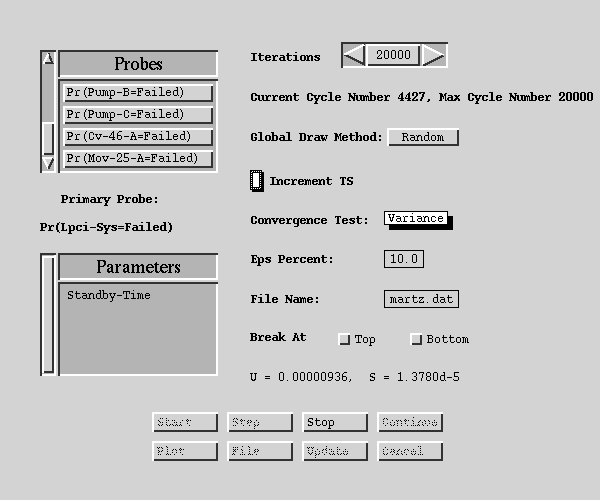
Figure 9. Simulation Controller. U and S are mean and variance of
observed system failure rate.
The simulation controller allows us to do just that. Using the simulation controller, we select a number of probes to monitor and start drawing from the distribution. Before we turn the controller on, the system shows the "nominal" rate, this is what Graphical-Belief uses for its default calculations. In the nominal rate, we use the expected value for each unknown parameter which has a law (if the law doesn't have an expectation, we use the median instead). We have already observed the nominal failure rate, it is 4.045e-6.
When we turn on the simulation controller we get the system failure rate estimate 9.329e-6 (with a standard error of 0.182e-6 after 5300) iterations. This is actually a sample of size 5300 from the distribution of the system failure rate. We can also calculate is quantiles. The median system failure rate is 4.921e-6, the 95% upper bound is 3.20e-5 and the 5% lower bound is 1.57e-7. These agree well with the estimates found in Martz and Waller [1990].
The difference between the nominal estimate (4.045e-6) and the Monte Carlo estimate (9.329e-6) shows that global dependence is an important phenomenon and cannot be ignored. It is closely related to the idea of a common cause failure (a single event on which many other events depend) which is the next example.
We can also perform similar calculations with second order belief function models, provided the modes are sufficiently well behaved. Almond [1995] discusses this phenomenon and its impact on belief function models in more detail.
In this example, we explored how Graphical-Belief uses parameters and laws to build second order model of uncertainty. The big advantage of the second order model is that it can be updated with new data. The example above shows how easy it is, the analyst just records the data on a form such as Figure 5.
We also saw how object--oriented model construction simplifies the construction of complex global dependencies. The next example explores the model construction features of Graphical-Belief.
 Construction. Continue with this
example and explore the implication of loops in the graphical model.
This example also shows how the model construction features work.
Construction. Continue with this
example and explore the implication of loops in the graphical model.
This example also shows how the model construction features work.
 Return to
the main example page.
Return to
the main example page.
Back to overview of Graphical-Belief.
 View a list
of Graphical-Belief in publications and downloadable technical
reports.
View a list
of Graphical-Belief in publications and downloadable technical
reports.
 The Graphical-Belief user
interface is implemented in Garnet.
The Graphical-Belief user
interface is implemented in Garnet.
 Get more
information about obtaining Graphical-Belief (and why
it is not generally available).
Get more
information about obtaining Graphical-Belief (and why
it is not generally available).
 get
the home page for Russell Almond , author
of Graphical-Belief.
get
the home page for Russell Almond , author
of Graphical-Belief.
![]() Click
here to get to the home page for Insightful (the company that StatSci
has eventually evolved into).
Click
here to get to the home page for Insightful (the company that StatSci
has eventually evolved into).